import numpy as np
from math import *
import drawMesh
import pygmsh
import gmshThe finite element method is a numerical technique used to solve complex engineering and physical problems. It is a powerful tool that allows for the accurate prediction of the behavior of a system under a wide range of conditions, making it an essential tool for engineers and scientists working in fields such as structural analysis, fluid dynamics, and electromagnetics. In this blog post, we will explore the basics of the finite element method and how it is used to solve real-world problems using Python. Whether you are an experienced engineer or a curious learner, I hope that this post will provide you with a better understanding of this important and versatile method.
By the end of this tutorial, you will be able to use Python to implement the finite element method and apply it to solve simple problems.
All the code can be found here.
Introduction
The Finite Element Method works by dividing a physical space into different elements and applying the governing equations to each element. This is very useful for complex geometries or boundary conditions were obtaining an analytical expression is not feasible.
Although FEM can be applied for many different physical problems, it is more commonly used in structural analysis. Therefore will be developing the FEM for structural analysis in 2D. In this example the structural case will be a 2D rectangular plate (\(3m \times 10m\)) with an hole of \(1m\) of diameter, fixed on one side and subjected to a constant tension force of \(1 \hspace{1mm} kN\) on the opposite side:
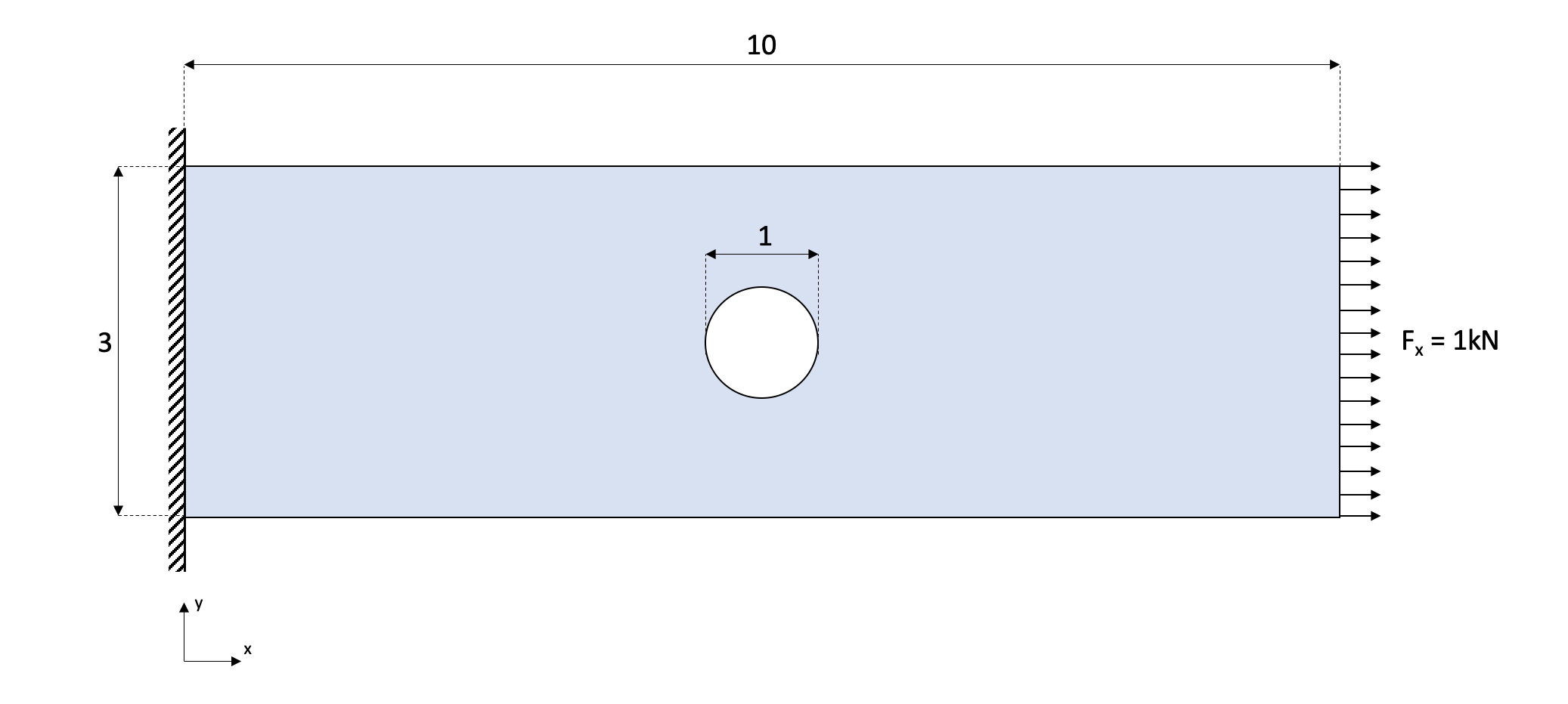
To simplify the calculations, 3-node triangular elements will be used.
The main equation in the FEM for structural analysis is the following: \[\textbf{K} \textbf{d} = \textbf{F}\] Where \(\textbf{d}\) is the displacement vector, \(\textbf{F}\) is the force vector and \(\textbf{K}\) is the stiffness matrix. The displacement vector contains the displacements of the nodes, the force vector is composed by the external forces and the reaction forces of the nodes. For the rest of the tutorial the force vector will be expressed as the sum of the external forces (\(\textbf{f}\)) and the reaction forces (\(\textbf{r}\)): \[\textbf{K} \textbf{d} = \textbf{f} + \textbf{r}\]
While the displacements and forces seem quite intuitive to understand, the stiffness matrix is a bit more abstract. It can be understood as the resistance to deformation. It is analogous to the spring constant (\(k\)) in Hooke’s law:

Requirements
To run this code some libraries are required:
Terminal
pip install numpyTerminal
pip install pygmshTerminal
pip install gmshTerminal
pip install pygletTo start we must import some libraries, including numpy, pygmsh, drawMesh and gmsh. NumPy is a library for scientific computing in Python, and is often used for numerical calculations and data manipulation. The math library provides mathematical functions. The library drawMesh is a simple mesh visualization library based on pyglet developed for this project, it can be found in the github repository. Finally, gmsh is a powerful mesh generation software that can be used in conjunction with pygmsh. Together, these libraries provide the tools necessary to implement the finite element method in Python.
Mesh
The splitting of the geometry into elements and nodes can be done manually but it becomes exponentially difficult for complex geometries and finer mesh resolutions. Therefore we make use of gmsh, a powerful meshing tool.
We create the mesh using pygmsh. The mesh resolution is defined in the variable resolution. The lower the value of resolution, the more the mesh will be divided into elements. This will lead to better results but higher computational cost. One of the key decisions when working with the FEM is to balance between mesh resolution and computing power.
gmsh.initialize()
rect_width, rect_length  = 3.0, 10.0
resolution = 0.1
geom = pygmsh.geo.Geometry()

circle = geom.add_circle([5,1.5,0], radius=0.5, mesh_size=resolution*0.5, make_surface=False)

rect = geom.add_polygon(
    [
        [0.0, 0.0                ,0],
        [0.0, rect_width         ,0],
        [rect_length, rect_width ,0],
        [rect_length, 0.0        ,0],
    ],
    mesh_size=resolution , holes = [circle]

)

mesh = geom.generate_mesh(dim=2)
geom.__exit__()
The resultant mesh looks like this:
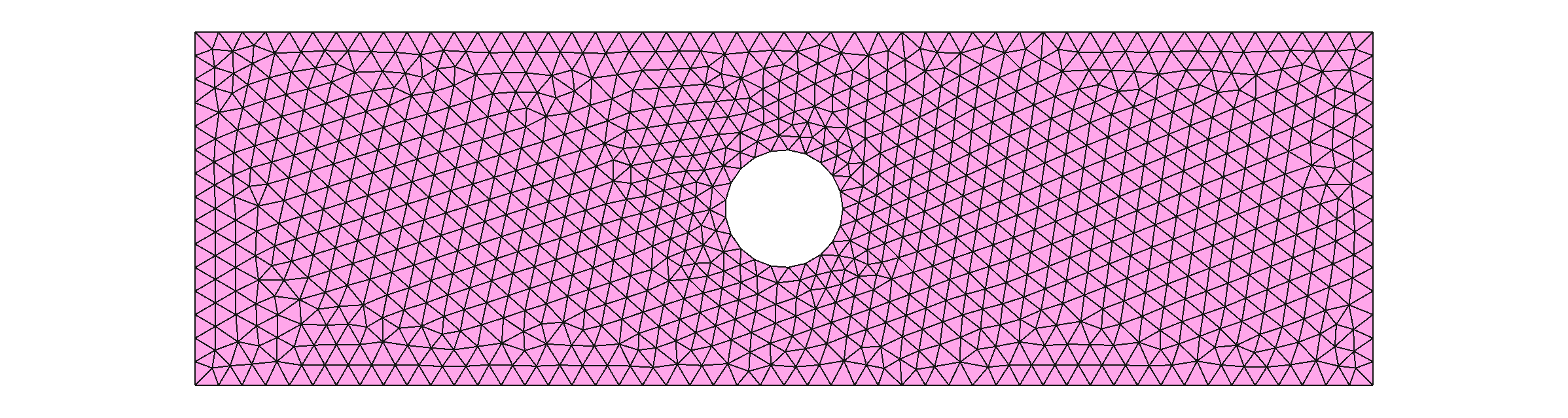
This mesh is composed of many nodes, that form triangular elements. Some nodes are shared by different elements.
Node
The following code defines the Node class, which represents a node in a mesh. The class has several attributes and methods that are used to store and manipulate information about the node, such as its coordinates, forces, and displacements.
The init method is used to initialize a new Node object, and accepts the node’s id, x and y coordinates as arguments. The fx and fy attributes are used to store the external forces applied to the node, and the rx and ry attributes are used to store the reaction forces at the node. The dx and dy attributes are used to store the displacements of the node.
The dfix property returns a boolean value indicating whether the node is fixed in both x and y directions. The externalForce property returns a boolean value indicating whether the node has any external forces applied to it. The __eq__ method is used to compare two Node objects and returns a boolean value indicating whether they are at the same location. This class can be used to represent nodes in a mesh and perform operations on them.
class Node:

    def __init__(self, id, x, y):
        self.id = id
        self.x, self.y = x, y
        self.fx, self.fy = 0.0, 0.0
        self.rx, self.ry = 0.0 ,0.0
        self.dx, self.dy = None, None

    @property
    def dfix(self):
        if self.dx == 0.0 and self.dy == 0.0:
            return True
        else:
            return False

    @property
    def externalForce(self):
        if self.fx != 0.0 or self.fy != 0.0:
            return True
        else:
            return False

    def __eq__(self, obj):
        if (self.x == obj.x) and (self.y == obj.y):
            return True
        else:
            return False
Element
Each element contains a series of nodes. In this case, we are using triangular nodes therefore each element has three nodes. It is important for the calculations that the nodes in each element are ordered counter-clockwise, therefore the passed nodes in the initialization are ordered with the orderCounterClock() method. The getArea()method calculates the area of the element. Each element contains a stress (\(\vec{\sigma}\)) and a strain (\(\vec{\varepsilon}\)) attributes:
\[ \vec{\sigma} = \begin{bmatrix} \sigma_{xx}\\ \sigma_{yy}\\ \sigma_{xy}\\ \end{bmatrix} \hspace{10mm} \vec{\varepsilon} = \begin{bmatrix} \varepsilon_{xx}\\ \varepsilon_{yy}\\ \gamma_{xy}\\ \end{bmatrix} \]
The getColormethod takes the colorVal variable and returns a RGB color taking in account the maximum and minimum colorVal of the elements. The colorFuncis used to interpolate the colors and the values, by default it is a linear function, but in some cases it may be useful to have a logarithmic interpolation instead for example.
class Element:

    maxColorVal = -9.9e19
    minColorVal = 9.9e19
    colorFunc = lambda x: x

    def __init__(self, id, nodes):
        self.id = id
        self.nodes = self.orderCounterClock(nodes)
        self.stress = None
        self.strain = None
        self.colorVal = 0
        self.getArea()

    @property
    def getmaxColorVal(self):
        return Element.maxColorVal

    @property
    def getminColorVal(self):
        return Element.minColorVal

    @property
    def getcolorFunc(self):
        return Element.colorFunc

    def getde(self):
        de_ = []
        for n in self.nodes:
            de_.append(n.dx)
            de_.append(n.dy)
        self.de = np.array(de_)
        return self.de

    def getColor(self):

        try: x_ = float(self.colorVal - Element.minColorVal)/(Element.maxColorVal - Element.minColorVal)
        except ZeroDivisionError: x_ = 0.5 # cmax == cmin

        x = Element.colorFunc(x_)

        blue  = int(255* min((max((4*(0.75-x), 0.)), 1.)))
        red   = int(255* min((max((4*(x-0.25), 0.)), 1.)))
        green = int(255* min((max((4*fabs(x-0.5)-1., 0.)), 1.)))
        return (red, green, blue)

    def getArea(self):
        x1,y1 = self.nodes[0].x, self.nodes[0].y
        x2,y2 = self.nodes[1].x, self.nodes[1].y
        x3,y3 = self.nodes[2].x, self.nodes[2].y
        result = 0.5*((x2*y3 - x3*y2)-(x1*y3- x3*y1)+(x1*y2-x2*y1))
        if result == 0:
            result = 1e-20
        self.area = result
        return result

    def getBe(self):
        x1,y1 = self.nodes[0].x, self.nodes[0].y
        x2,y2 = self.nodes[1].x, self.nodes[1].y
        x3,y3 = self.nodes[2].x, self.nodes[2].y
        B = (0.5/self.area) * np.array([
            [(y2-y3) ,  0    , (y3-y1),  0   ,   (y1-y2),   0   ],
            [   0    , (x3-x2),  0    , (x1-x3),     0   ,(x2-x1)],
            [(x3-x2) , (y2-y3), (x1-x3), (y3-y1), (x2-x1) ,(y1-y2)],
        ], dtype=np.float64)
        self.Be = B
        return B

    def getKe(self, D):
        Bie = self.getBe()
        Ke = self.area* np.matmul(Bie.T, np.matmul(D, Bie))
        self.Ke = Ke
        return Ke

    def orderCounterClock(self, nodes):
        p1,p2,p3 = nodes[0], nodes[1], nodes[2]
        val = (p2.y - p1.y) * (p3.x - p2.x) - (p2.x - p1.x) * (p3.y - p2.y)
        nodes_ = nodes.copy()
        if val > 0:
            nodes[1] = nodes_[0]
            nodes[0] = nodes_[1]

        assembly = []
        for n in nodes:
            assembly.append(int(n.id*2))
            assembly.append(int(n.id*2) +1)
        self.assembly = assembly

        return nodes
It is important to make the distinction between global and local variables and clarify the notation. Element numbers are denoted with a superscript and node numbers are denoted with a subscript. When a variable does not have a superscript is a global variable. For example, the local point \(0\) of the element number \(4\) is denoted as \(P_0^{(4)}\). Note the difference between a local and global point, \(P_0^{e} \ne P_0\).
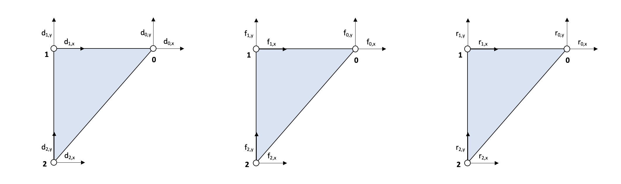
The force-displacement equation for an element is: \(\mathbf{K^e} \mathbf{d^e} = \mathbf{f^e} + \mathbf{r^e}\), where the displacements vector (\(\mathbf{d^e}\)), and stiffness matrix (\(\mathbf{K^e}\)) have the following form:
\[\begin{equation} \mathbf{d^e} = \begin{bmatrix} d_{0,x}^e\\ d_{0,y}^e\\ d_{1,x}^e\\ d_{1,y}^e\\ d_{2,x}^e\\ d_{2,y}^e\\ \end{bmatrix} \hspace{10mm} \mathbf{K^e} = \begin{bmatrix} k_{00} & k_{01} & k_{02} & k_{03} & k_{04} & k_{05} & \\ k_{10} & k_{11} & k_{12} & k_{13} & k_{14} & k_{15} & \\ k_{20} & k_{21} & k_{22} & k_{23} & k_{24} & k_{25} & \\ k_{30} & k_{31} & k_{32} & k_{33} & k_{34} & k_{35} & \\ k_{40} & k_{41} & k_{42} & k_{43} & k_{44} & k_{45} & \\ k_{50} & k_{51} & k_{52} & k_{53} & k_{54} & k_{55} & \\ \end{bmatrix} \end{equation}\]
The stiffness matrix for each element can be obtained deriving the weak form of the elasticity problem (see Fish and Belytschko 2007, 227), resulting in the following equation: \[ \mathbf{K^e} = \int_{\Omega}(\mathbf{B^e})^T \mathbf{D} \hspace{1mm} \mathbf{B^e} d \Omega \] The Hookean matrix \(\mathbf{D}\) will be discussed later on, but basically, it relates the strain and stresses taking in account the material properties. The matrix \(\mathbf{B^e}\) is a bit more complex, but the main thing to understand is that it relates the displacements at the nodes of an element to the gradient of the displacement function \(\theta^e(x,y)\) (see Fish and Belytschko 2007, 78–84).
\[ \nabla \theta^e = \mathbf{B}^e \mathbf{d}^e \]
The displacement function can be understood as an interpolation of the node displacements across the space of the element. This can be any arbitrary polynomial function such that at the nodes the function matches the displacement, and that the continuity condition is meet at the boundaries of the elements.
\[ \theta^e(x_0,y_0) = \begin{bmatrix} d_{x,0} \\ d_{y,0}\end{bmatrix} \]
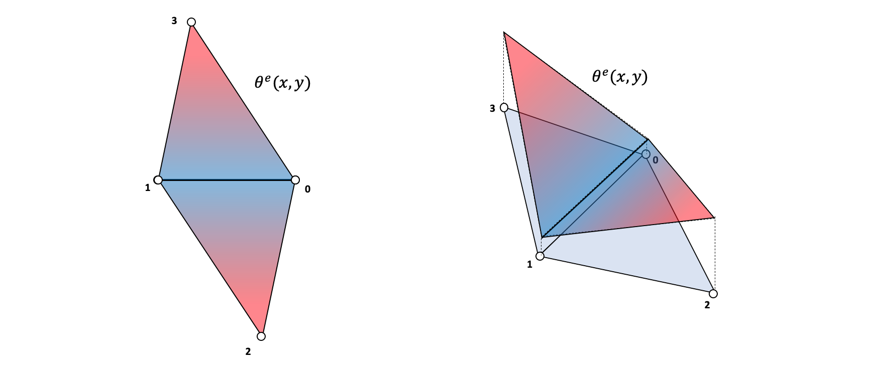
For simplification purposes in this tutorial we will use a three-node linear function which yields the following formula to construct the \(\mathbf{B^e}\) matrix (see Fish and Belytschko 2007, 160).
\[\begin{equation} \mathbf{B^e} = \frac{1}{2 A^e} \begin{bmatrix} (y_1^e - y_2^e) & 0 & (y_2^e - y_0^e) & 0 & (y_0^e - y_1^e) & 0 & \\ 0 & (x_2^e - x_1^e) & 0 & (x_0^e - x_2^e) & 0 & (x_1^e - x_0^e) & \\ (x_2^e - x_1^e) & (y_1^e - y_2^e) & (x_0^e - x_2^e) & (y_2^e - y_0^e) & (x_1^e - x_0^e) & (y_0^e - y_1^e) & \\ \end{bmatrix} \end{equation}\]
This choice of the linear function results in a \(\mathbf{B^e}\) matrix that is constant along the surface (\(\Omega\)) of the element, therefore we can simplify the weak form equation to obtain the element stiffness matrix:
\[ \mathbf{K^e} = (\mathbf{B^e})^T \mathbf{D} \hspace{1mm} \mathbf{B^e} \]
Preprocessing
Extracting mesh data
The mesh contains points and cells data. Each data row in the cells array contains the index of the three points of a cell or element.
\[ \textbf{cells} = \begin{bmatrix} P_0^{(0)} & P_1^{(0)} & P_2^{(0)} \\ P_0^{(1)} & P_1^{(1)} & P_2^{(1)} \\ \vdots & \vdots & \vdots \\ P_0^{(N_{el})} & P_1^{(N_{el})} & P_2^{(N_{el})} \\ \end{bmatrix} \hspace{10mm} \textbf{points} = \begin{bmatrix} P_0 \\ P_1 \\ \vdots \\ P_{N_{n}} \end{bmatrix} \hspace{10mm} P_i = \begin{bmatrix} x_i & y_i \end{bmatrix} \]
- \(N_{el}\) : Number of elements
- \(N_{n}\) : Number of nodes (or points)
Because of how the pygmsh library works, the mesh starts counting points including some points like the center of the circle that are not exported to the mesh. Therefore the numbering of the nodes must be modified so that the first point in the mesh is numbered as \(0\):
maxNode = 0
for cell in mesh.cells[1].data:
    for node in cell:
        if node > maxNode:
            maxNode = node

meshCells = mesh.cells[1].data - np.full(np.shape(mesh.cells[1].data), 1, dtype=np.uint64)
meshPoints = mesh.points[1:]
Next, the elements and nodes are generated and stored in the lists elements and nodesrespectively:
nodes = [Node(i, point[0], point[1]) for i, point in enumerate(meshPoints)]
elements = []

for i,cell in enumerate(meshCells):
    elements.append(
        Element(id=i, nodes=[nodes[i] for i in cell])
    )
Material properties
As mentioned before the \(\mathbf{D}\) matrix relates the stress and strains of an element. The Hookean matrix can be calculated with the Young’s modulus (\(E\)) and Poisson’s ratio (\(\nu\)):
\[ \mathbf{D} = \frac{E}{1-\nu^2} \begin{bmatrix} 1 & \nu & 0 \\ \nu & 1 & 0 \\ 0 & 0 & \frac{1}{2}(1-\nu) \\ \end{bmatrix} \]
For this example lets use the material properties of steel.
v = 0.28        # Poisson ratio of steel
E = 200.0e9     # Young modulus of steel

D = (E/(1-v**2)) * np.array([
    [1, v, 0],
    [v, 1, 0],
    [0, 0, (1-v)/2],
])
Boundary conditions
Once the mesh and material properties are defined the next step is to define the boundary conditions, external forces, reaction forces and unknowns. The unknown variables, i.e variables to solve for, are defined by assigning the None value. All the displacements are None by default, and all the external and reaction forces are 0.0 by default.
for i, node in enumerate(nodes):
    if node.x == rect_length:           # At right side of the rectangle (x=10)
        node.fx = 1.0e3                 # Apply a tension force in the x direction of 1kN
    elif node.x == 0.0:                 # At left side of the rectangle (x=0)
        node.dx, node.dy = 0.0, 0.0     # Fix the displacement in x and y
        node.rx, node.ry = None, None   # Set the reaction forces as unknowns
Matrix assembly
Now that the mesh and case conditions are defined the \(\mathbf{K}\) matrix must be obtained to solve the displacements-forces equation. The global stiffness matrix can be obtained as the sum of the element stiffness matrices \(\mathbf{\hat{K}^e}\).
\[ \mathbf{K} = \sum_{i = 0}^{N_{el}} \mathbf{\hat{K}^e} \]
Note that \(\mathbf{\hat{K}^e} \ne \mathbf{K^e}\). The local stiffness matrix of an element (\(\mathbf{K^e}\)) has a shape of \((6 \times 6)\) while the global stiffness matrix of an element (\(\mathbf{\hat{K}^e}\)) has a shape of \((2 N_{n} \times 2 N_{n})\). Therefore we need a function that map each element’s local stiffness matrix to the global one.
\[ \textnormal{assemblyK}\left(\mathbf{K^e} \right) = \mathbf{\hat{K}^e} \]
The assemblyK function takes as arguments the global total stiffness matrix and the nodeAssembly, and adds to \(\mathbf{K}\) the element stiffness matrix:
def assemblyK(K, Ke, nodeAssembly):
    for i,t in enumerate(nodeAssembly):
        for j,s in enumerate(nodeAssembly):
            K[t][s] += Ke[i][j]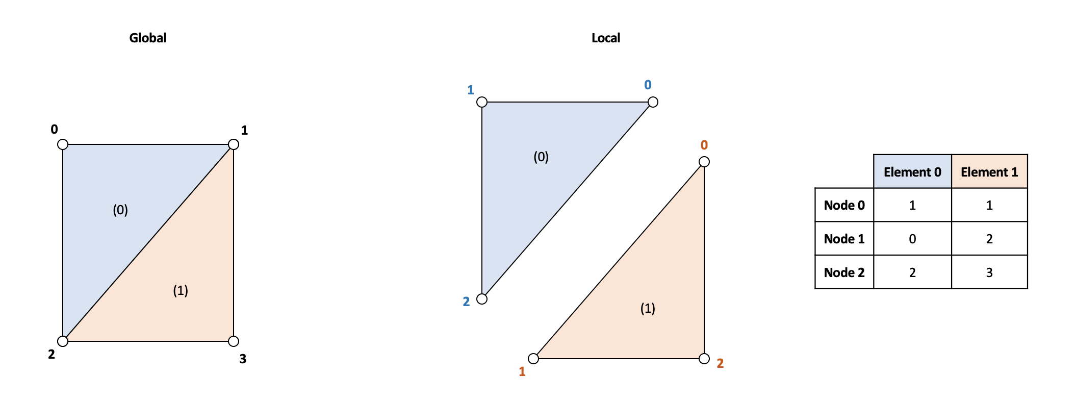
The following code iterates throughout all the elements and sums the stiffness matrix. Each element has an attribute assembly that contains the relations between the local position of the nodes in the element to the global position of the node.
Nnodes = len(nodes)
K = np.zeros((Nnodes*2,Nnodes*2))

for e in elements:
    Ke = e.getKe(D)
    nodeAssembly = e.assembly
    assemblyK(K, Ke, nodeAssembly)
Now we have the matrix \(\mathbf{K}\) but we need to create and fill in the forces, reactions and displacements vectors with the values of the nodes so that the problem can be solved using the numpylibrary. As some nodes have unknown values we create the lists rowsrk and rowsdk that store the rows where the reaction forces are known and the displacements are known respectively.
f = np.zeros((int(2*Nnodes), 1))        # Forces vector
d = np.full((int(2*Nnodes), 1), None)   # Displacements vector
r = np.full((int(2*Nnodes), 1), None)   # Recation forces vector

rowsrk, rowsdk = [], []                 # Known reactions rows, Known displacements rows

for i,node in enumerate(nodes):
    ix,iy = int(i*2), int(i*2)+1

    f[ix], f[iy] = node.fx, node.fy
    d[ix], d[iy] = node.dx, node.dy
    r[ix], r[iy] = node.rx, node.ry

    if node.dx == None:
        rowsrk.append(ix)
    else:
        rowsdk.append(ix)

    if node.dy == None:
        rowsrk.append(iy)
    else:
        rowsdk.append(iy)
Solver
Now that we have the stiffness matrix (\(\mathbf{K}\)), forces vector (\(\mathbf{f}\)), reactions vector (\(\mathbf{r}\)) and displacements vector (\(\mathbf{d}\)), we must organize this vectors and matrices by the known and unknown variables in such a way that can be solved. For example, in the following equation, \(d_1\), \(d_2\) and \(r_0\) are unknowns: \[\begin{equation} \begin{bmatrix} k_{00} & k_{01} & k_{02} \\ k_{10} & k_{11} & k_{12} \\ k_{20} & k_{21} & k_{22} \\ \end{bmatrix} \begin{bmatrix} 0 \\ d_1 \\ d_2 \\ \end{bmatrix} = \begin{bmatrix} r_0 \\ -4 \\ 10 \\ \end{bmatrix} \end{equation}\]
The matrix system of equations can be partitioned in such a way that we can separate the unknowns and knowns in the forces and displacements vectors. So \(\mathbf{d_K}\) is the vector of known displacements and \(\mathbf{d_U}\) the vector of unknowns. The same is done to obtain the forces vectors \(\mathbf{f_K}\) and \(\mathbf{f_U}\).
\[\begin{equation} \mathbf{f_U} = \begin{bmatrix} r_0 \\ \end{bmatrix} \hspace{5mm} \mathbf{d_U} = \begin{bmatrix} d_1 \\ d_2 \\ \end{bmatrix} \hspace{5mm} \mathbf{f_K} = \begin{bmatrix} -4 \\ 10 \\ \end{bmatrix} \hspace{5mm} \mathbf{d_K} = \begin{bmatrix} 0 \\ \end{bmatrix} \end{equation}\]
We can then rewrite the system of equations:
\[\begin{equation} \begin{bmatrix} \mathbf{K_{A}} & \mathbf{K_{AB}} \\ \mathbf{K_{AB}^T} & \mathbf{K_{B}} \\ \end{bmatrix} \begin{bmatrix} \mathbf{d_K}\\ \mathbf{d_U} \\ \end{bmatrix} = \begin{bmatrix} \mathbf{f_U} \\ \mathbf{f_K} \\ \end{bmatrix} \end{equation}\]
From this matrix equation we can separate the knows and unknowns to get a set of equations to solve for the unknowns. Because the known displacements are null, we can further simplify the equations:
\[ \mathbf{f_U} = \mathbf{K_A} \mathbf{d_K} + \mathbf{K_{AB}} \mathbf{d_U} = \mathbf{K_{AB}} \mathbf{d_U} \]
\[ \mathbf{f_K} = \mathbf{K_{AB}^T} \mathbf{d_K} + \mathbf{K_B} \mathbf{d_U} = \mathbf{K_B} \mathbf{d_U} \]
In the following code this matrices are constructed such that, \(\mathbf{K_B}_{i,j} = \mathbf{K}_{t,t}\) and \(\mathbf{K_A}_{i,j} = \mathbf{K}_{s,t}\), where \(t\) and \(s\) are the indexes of the rows of the unknown reactions and displacements respectively.
KB = np.zeros((len(rowsrk),len(rowsrk)))
KA = np.zeros((len(rowsdk),len(rowsrk)))

fk = np.array([r[i] for i in rowsrk]) + np.array([f[i] for i in rowsrk])
dk = np.array([d[i] for i in rowsdk])

for i in range(np.shape(KB)[0]):
    for j in range(np.shape(KB)[1]):
        KB[i][j] = K [rowsrk[i]][rowsrk[j]]

for i in range(np.shape(KA)[0]):
    for j in range(np.shape(KA)[1]):
        KA[i][j] = K [rowsdk[i]][rowsrk[j]]
The previous equations can be then rearranged to solve for the unknown displacements and forces: \[ \mathbf{d_U} = \mathbf{K_B}^{-1} \mathbf{f_K} \hspace{30mm} \mathbf{f_U} = \mathbf{K_A} \mathbf{d_U} \]
Using the linalg.invfunction of numpy the matrix \(\mathbf{K_B}\) is inverted. This operation is computationally expensive and grows with the number of nodes. There are other algorithms like the LU decomposition that can improve the performance of this calculation, but for the sake of simplicity we will stick with the matrix inversion.
du = np.matmul(np.linalg.inv(KB), fk)
fu = np.matmul(KA,du)
Postprocessing
Now that we have solved the problem, the only thing left is to restructure and visualize the results. We take the solved displacements stored in du and assign them to the correspondent position in the final displacement vector d_total:
d_total = d.copy()

for i, d_solve in zip(rowsrk, du):
    d_total[i] = d_solve
Next we assign the final displacement values to the correspondent nodes:
for i,n in enumerate(nodes):
    ix,iy = int(i*2), int(i*2)+1
    n.dx = d_total[ix][0]
    n.dy = d_total[iy][0]
von Mises stress
The von Mises yield criterion is a very good way to estimate when an element will undergo plastic deformation by comparing the von Mises stress equivalent to the critical yield stress of the material. The von Mises equivalent stress can be calculated with the following equation: \[ \sigma_v = \sqrt{\sigma_{xx} + \sigma_{yy} + 3\sigma_{xy}^2 - \sigma_{xx}\sigma_{yy} } \]
def calculateVonMises(sx, sy, sxy):
    return sqrt(sx**2 + sy**2 + 3*(sxy**2) - sx*sy)
Visual representation
The rgb function interpolates an input value between a maximum and minimum and returns a specific RGB color. The lower values are light blues and the higher are reds and yellows.
def rgb(mag, cmin, cmax):
    try: x = float(mag-cmin)/(cmax-cmin)
    except ZeroDivisionError: x = 0.5

    blue  = int(255* min((max((4*(0.75-x), 0.)), 1.)))
    red   = int(255* min((max((4*(x-0.25), 0.)), 1.)))
    green = int(255* min((max((4*fabs(x-0.5)-1., 0.)), 1.)))
    return (red, green, blue)

average = lambda x: (sum(x)/len(x))
The static attribute colorFunc of the Element class defines the function used to interpolate the values to the color. Here we set it to a linear function but it can be changed to an logarithmic function for example.
maxd, mind = max(d_total)[0], min(d_total)[0]
Element.colorFunc = lambda x: x # Logarithmic: exp(-x)
The stresses are calculated using the generalized Hook’s expression. \[ \varepsilon^e = \mathbf{B}^e \mathbf{d}^e \hspace{20mm} \sigma^e = \mathbf{D} \varepsilon^e \]
The strains and stresses are calculated for each element and the color of each element is assigned depending on the value of the von Mises stress. The colorVal determines the value used for coloring, this can be modified so that the strains are colored instead for example.
for i,element in enumerate(elements):

    de = element.getde()
    strain_e = np.matmul(element.Be, de)
    stress_e = np.matmul(D, strain_e)

    element.strain = strain_e
    element.stress = stress_e

    element.colorVal = calculateVonMises(element.stress[0], element.stress[1], element.stress[2])

    if element.colorVal > Element.maxColorVal:
        Element.maxColorVal = element.colorVal
    if element.colorVal < Element.minColorVal:
        Element.minColorVal = element.colorVal
Finally the results are viewed using the drawMesh module:
render = drawMesh.MeshRender()          # Creates an instance of a MeshRender
render.legend = True                    # The legened will be drawn
render.autoScale = True                 # The mesh will be automatically scaled to fit the window
render.deform_scale = 1.0e5             # Sets the scale to draw the deformation of the nodes displacement
render.legendTitle = 'von-mises (Pa)'
render.drawElements(elements)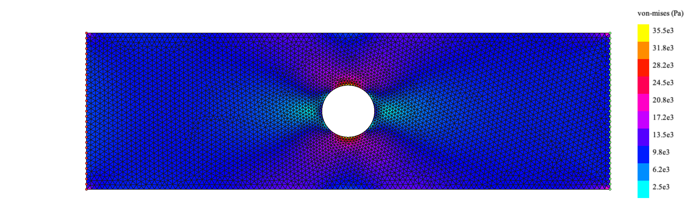
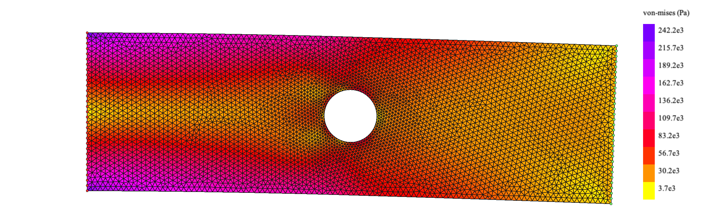
If we rerun the code changing the force direction downwards we get the following result:
This particular problem of a plate with a hole in tension has been studied thoroughly due to its implications regarding riveting, aircraft pressurization and many other applications. There is an analytical expression to calculate the stresses in polar coordinates in a rectangular plate with a hole of radius \(R\) subjected to a tensional stress at both ends of \(\sigma_t\):
\[ \sigma_r(r, \theta) = \frac{\sigma_t}{2} \left( 1- \frac{R^2}{r^2} \right) + \frac{\sigma_t}{2} \left( 1 + 3\frac{R^4}{r^4} - 4 \frac{R^2}{r^2} \right) \cos(2\theta) \]
\[ \sigma_{\theta}(r, \theta) = \frac{\sigma_t}{2} \left( 1 + \frac{R^2}{r^2} \right) - \frac{\sigma_t}{2} \left( 1 + 3\frac{R^4}{r^4} \right) \cos(2\theta) \]
\[ \tau_{r\theta}(r, \theta) = -\frac{\sigma_t}{2} \left( 1 - 3\frac{R^4}{r^4} + 2\frac{R^2}{r^2} \right) \sin(2\theta) \]
Calculating the von Mises stress and plotting the analytical expression using the same values as the example, yields the following result :
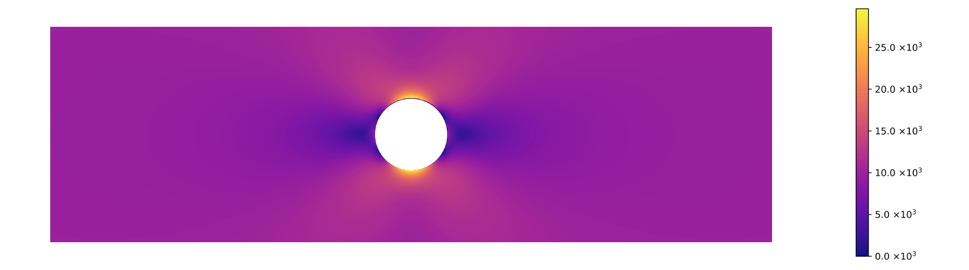
We can see that the results of the FEM method are the same as the predicted by the analytical method.
References
Fish, J., and Ted Belytschko. 2007. A First Course in Finite Elements. Chichester, England ; Hoboken, NJ: John Wiley & Sons Ltd.